
How to merge and clean up multiple CSVs using R
This tutorial solves a problem I was having when working through the exploratory data analysis exercises in Doing Data Science by Cathy O’Neil and Rachel Schutt. I highly recommended picking up a copy for yourself. The exercises in the book are intended for a single day, but what if I wanted to look at an entire month’s worth of data? Luckily, I remembered learning a handy workflow for processing multiple data files in the third ggplot2 course from Datacamp by Rick Scavetta.
If you have a situation where all your data files need similar wrangling/preparation before visualizing or modeling, you will find this helpful.
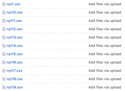
I’m starting with a folder that contains 31 CSVs, each with one day’s worth of simulated clicks for ads shown on The New York Times home page. Rows represent users, and the variables are: Age, Gender (0 = female, 1 = male), Impressions (number impressions), Clicks (number clicks), and a binary indicator for signed in or not Signed_in.
Towards the end of the tutorial, I will create two new variables: age_group, which contains six levels of Age (“<18”, “18-24”, “25-34”, “35-44”, “45-54”, “55-64”, and “65+”), and CTR or clickthrough-rate, calculated as the number of clicks / the number of impressions.
Data files
I’ve moved the data from the Github repository to a local data folder (./data/).
Read data files
I will start by reading the first data set into RStudio using readr::read_csv() and then use dplyr::glimpse() to see what these data look like.
nyt1 <- readr::read_csv(file = "./data/nyt1.csv",
                col_names = TRUE)
## Parsed with column specification:
## cols(
##   Age = col_integer(),
##   Gender = col_integer(),
##   Impressions = col_integer(),
##   Clicks = col_integer(),
##   Signed_In = col_integer()
## )
nyt1 %>% dplyr::glimpse()
## Observations: 458,441
## Variables: 5
## $ Age         <int> 36, 73, 30, 49, 47, 47, 0, 46, 16, 52, 0, 21, 0, 5...
## $ Gender      <int> 0, 1, 0, 1, 1, 0, 0, 0, 0, 0, 0, 0, 0, 0, 0, 0, 1,...
## $ Impressions <int> 3, 3, 3, 3, 11, 11, 7, 5, 3, 4, 8, 3, 4, 6, 5, 6, ...
## $ Clicks      <int> 0, 0, 0, 0, 0, 1, 1, 0, 0, 0, 1, 0, 0, 0, 0, 0, 0,...
## $ Signed_In   <int> 1, 1, 1, 1, 1, 1, 0, 1, 1, 1, 0, 1, 0, 1, 1, 0, 1,...
I see all 5 variables in this data frame. I will create a pipeline that creates the two variables from the exercises and a third Female variable that makes the categories in Gender less ambiguous. When I am done, I look at the data with dplyr::glimpse() again.
nyt1 <- nyt1 %>%
    dplyr::mutate(
        age_group = case_when( # create age_group variable
            Age < 18 ~ "<18",
            Age >= 18 & Age < 25 ~ "18-24",
            Age >= 25 & Age < 35 ~ "25-34",
            Age >= 35 & Age < 45 ~ "35-44",
            Age >= 45 & Age < 55 ~ "45-54",
            Age >= 55 & Age < 65 ~ "55-64",
            Age >= 65 ~ "65+"),
        CTR = Clicks/Impressions, # create CTR variable
        Female = case_when( # create new Female variable
            Gender == 0 ~ "Male",
            Gender == 1 ~ "Female",
            TRUE ~ as.character(Gender)))
nyt1 %>% dplyr::glimpse()
## Observations: 458,441
## Variables: 8
## $ Age         <int> 36, 73, 30, 49, 47, 47, 0, 46, 16, 52, 0, 21, 0, 5...
## $ Gender      <int> 0, 1, 0, 1, 1, 0, 0, 0, 0, 0, 0, 0, 0, 0, 0, 0, 1,...
## $ Impressions <int> 3, 3, 3, 3, 11, 11, 7, 5, 3, 4, 8, 3, 4, 6, 5, 6, ...
## $ Clicks      <int> 0, 0, 0, 0, 0, 1, 1, 0, 0, 0, 1, 0, 0, 0, 0, 0, 0,...
## $ Signed_In   <int> 1, 1, 1, 1, 1, 1, 0, 1, 1, 1, 0, 1, 0, 1, 1, 0, 1,...
## $ age_group   <chr> "35-44", "65+", "25-34", "45-54", "45-54", "45-54"...
## $ CTR         <dbl> 0.00000, 0.00000, 0.00000, 0.00000, 0.00000, 0.090...
## $ Female      <chr> "Male", "Female", "Male", "Female", "Female", "Mal...
Now I want to bundle the data reading and preparing commands as a function, clean_nyt.
clean_nyt <- function(file) {
                    nyt <- read_csv(file)
                    nyt %>%
                    dplyr::mutate(
                        age_group = case_when( # create age_group variable
                                        Age < 18 ~ "<18",
                            Age >= 18 & Age < 25 ~ "18-24",
                            Age >= 25 & Age < 35 ~ "25-34",
                            Age >= 35 & Age < 45 ~ "35-44",
                            Age >= 45 & Age < 55 ~ "45-54",
                            Age >= 55 & Age < 65 ~ "55-64",
                            Age >= 65 ~ "65+"),
                        CTR = Clicks/Impressions, # create CTR variable
                        Female = case_when( # create new Female variable
                                Gender == 0 ~ "Male",
                                Gender == 1 ~ "Female",
                    TRUE ~ as.character(Gender)))
}
I will test clean_nyt() on a nyt2.csv
nyt2 <- clean_nyt("./data/nyt2.csv")
## Parsed with column specification:
## cols(
##   Age = col_integer(),
##   Gender = col_integer(),
##   Impressions = col_integer(),
##   Clicks = col_integer(),
##   Signed_In = col_integer()
## )
nyt2 %>% glimpse()
## Observations: 449,935
## Variables: 8
## $ Age         <int> 48, 0, 15, 0, 0, 0, 63, 0, 24, 16, 31, 0, 56, 52, ...
## $ Gender      <int> 1, 0, 1, 0, 0, 0, 0, 0, 1, 0, 1, 0, 1, 1, 1, 0, 1,...
## $ Impressions <int> 3, 9, 4, 5, 7, 11, 3, 4, 2, 7, 5, 3, 5, 6, 2, 5, 4...
## $ Clicks      <int> 0, 1, 0, 0, 1, 0, 0, 0, 0, 0, 0, 0, 0, 0, 0, 0, 0,...
## $ Signed_In   <int> 1, 0, 1, 0, 0, 0, 1, 0, 1, 1, 1, 0, 1, 1, 1, 1, 1,...
## $ age_group   <chr> "45-54", "<18", "<18", "<18", "<18", "<18", "55-64...
## $ CTR         <dbl> 0.0000, 0.1111, 0.0000, 0.0000, 0.1429, 0.0000, 0....
## $ Female      <chr> "Female", "Male", "Female", "Male", "Male", "Male"...
It looks like clean_nyt() is working!
Now I need to create a vector with the files in dir("./data"). I will call this nyt_files. Then I will paste0() the file path to the files and store this in the my_nyt_files vector.
nyt_files <- dir("./data")
my_nyt_files <- paste0("./data/",nyt_files)
my_nyt_files %>% head()
## [1] "./data/nyt1.csv"  "./data/nyt10.csv" "./data/nyt11.csv"
## [4] "./data/nyt12.csv" "./data/nyt13.csv" "./data/nyt14.csv"
Great. Now I can create a for loop to pass the files through and build a master data frame, my_nyt_data.
# Build my_nyt_data with a for loop
my_nyt_data <- NULL
for (file in my_nyt_files) { # for every file...
    temp <- clean_nyt(file)  # clean it with clean_nyt()
    temp$id <- sub(".csv", "", file) # add an id column (but remove .csv)
    my_nyt_data <- rbind(my_nyt_data, temp) # then stick together by rows
}
my_nyt_data %>% glimpse()
## Observations: 14,905,865
## Variables: 9
## $ Age         <int> 36, 73, 30, 49, 47, 47, 0, 46, 16, 52, 0, 21, 0, 5...
## $ Gender      <int> 0, 1, 0, 1, 1, 0, 0, 0, 0, 0, 0, 0, 0, 0, 0, 0, 1,...
## $ Impressions <int> 3, 3, 3, 3, 11, 11, 7, 5, 3, 4, 8, 3, 4, 6, 5, 6, ...
## $ Clicks      <int> 0, 0, 0, 0, 0, 1, 1, 0, 0, 0, 1, 0, 0, 0, 0, 0, 0,...
## $ Signed_In   <int> 1, 1, 1, 1, 1, 1, 0, 1, 1, 1, 0, 1, 0, 1, 1, 0, 1,...
## $ age_group   <chr> "35-44", "65+", "25-34", "45-54", "45-54", "45-54"...
## $ CTR         <dbl> 0.00000, 0.00000, 0.00000, 0.00000, 0.00000, 0.090...
## $ Female      <chr> "Male", "Female", "Male", "Female", "Female", "Mal...
## $ id          <chr> "./data/nyt1", "./data/nyt1", "./data/nyt1", "./da...
That is a big data set–14,905,865 observations and 9 variables.
Clean up id
Now we just need to clean up the id variable a little with the stringr::str_replace() function and verify all 31 data sets are accounted for using dplyr::distinct() and base::nrow().
my_nyt_data <- my_nyt_data %>%
    dplyr::mutate(id =
                      stringr::str_replace(id,
                                pattern = "./data/" ,
                                replacement = ""))
my_nyt_data %>%
    dplyr::distinct(id) %>%
    base::nrow()
## [1] 31
Check age_group
Ok we should check our new variables, age_group and Female. Let’s start with age_group using a combination of dplyr::count() and tidyr::spread().
my_nyt_data %>% dplyr::count(age_group, Age) %>%
    tidyr::spread(age_group, n) %>% head()
## # A tibble: 6 x 8
##     Age   `<18` `18-24` `25-34` `35-44` `45-54` `55-64` `65+`
##   <int>   <int>   <int>   <int>   <int>   <int>   <int> <int>
## 1     0 5613610      NA      NA      NA      NA      NA    NA
## 2     3       2      NA      NA      NA      NA      NA    NA
## 3     4       2      NA      NA      NA      NA      NA    NA
## 4     5      10      NA      NA      NA      NA      NA    NA
## 5     6      41      NA      NA      NA      NA      NA    NA
## 6     7     167      NA      NA      NA      NA      NA    NA
Yikes! There are 5613610 respondents with Age of 0. Let’s remove these using dplyr::filter() and re-check those zeros.
my_nyt_data <- my_nyt_data %>%
    filter(Age != 0)
my_nyt_data %>% count(age_group, Age) %>%
    spread(age_group, n) %>% head()
## # A tibble: 6 x 8
##     Age `<18` `18-24` `25-34` `35-44` `45-54` `55-64` `65+`
##   <int> <int>   <int>   <int>   <int>   <int>   <int> <int>
## 1     3     2      NA      NA      NA      NA      NA    NA
## 2     4     2      NA      NA      NA      NA      NA    NA
## 3     5    10      NA      NA      NA      NA      NA    NA
## 4     6    41      NA      NA      NA      NA      NA    NA
## 5     7   167      NA      NA      NA      NA      NA    NA
## 6     8   519      NA      NA      NA      NA      NA    NA
I should also check the top of the Age distribution with base::tail().
my_nyt_data %>% count(age_group, Age) %>%
    spread(age_group, n) %>% tail()
## # A tibble: 6 x 8
##     Age `<18` `18-24` `25-34` `35-44` `45-54` `55-64` `65+`
##   <int> <int>   <int>   <int>   <int>   <int>   <int> <int>
## 1   108    NA      NA      NA      NA      NA      NA     7
## 2   109    NA      NA      NA      NA      NA      NA     1
## 3   111    NA      NA      NA      NA      NA      NA     3
## 4   112    NA      NA      NA      NA      NA      NA     1
## 5   113    NA      NA      NA      NA      NA      NA     1
## 6   115    NA      NA      NA      NA      NA      NA     1
115 is old…but possible. Ok I also want to add the dplyr::filter(Age != 0) to the clean_nyt() function.
# update function
clean_nyt <- function(file) {
                    nyt <- readr::read_csv(file)
                    nyt %>%
                    dplyr::filter(Age != 0) %>%
                    dplyr::mutate(
                        age_group = case_when( # create age_group variable
                                        Age < 18 ~ "<18",
                            Age >= 18 & Age < 25 ~ "18-24",
                            Age >= 25 & Age < 35 ~ "25-34",
                            Age >= 35 & Age < 45 ~ "35-44",
                            Age >= 45 & Age < 55 ~ "45-54",
                            Age >= 55 & Age < 65 ~ "55-64",
                            Age >= 65 ~ "65+"),
                        CTR = Clicks/Impressions, # create CTR variable
                        Female = case_when( # create new Female variable
                                Gender == 0 ~ "Male",
                                Gender == 1 ~ "Female",
                    TRUE ~ as.character(Gender)))
}
Let’s re-run the for loop and make sure we have nice, clean data in my_nyt_data.
# Build my_nyt_data with a for loop
my_nyt_data <- NULL
for (file in my_nyt_files) { # for every file...
    temp <- clean_nyt(file)  # clean it with clean_nyt()
    temp$id <- sub(".csv", "", file) # add an id column (but remove .csv)
    my_nyt_data <- rbind(my_nyt_data, temp) # then stick together by rows
}
my_nyt_data %>% glimpse()
## Observations: 9,292,255
## Variables: 9
## $ Age         <int> 36, 73, 30, 49, 47, 47, 46, 16, 52, 21, 57, 31, 40...
## $ Gender      <int> 0, 1, 0, 1, 1, 0, 0, 0, 0, 0, 0, 0, 1, 1, 0, 1, 0,...
## $ Impressions <int> 3, 3, 3, 3, 11, 11, 5, 3, 4, 3, 6, 5, 3, 5, 4, 4, ...
## $ Clicks      <int> 0, 0, 0, 0, 0, 1, 0, 0, 0, 0, 0, 0, 0, 0, 0, 0, 0,...
## $ Signed_In   <int> 1, 1, 1, 1, 1, 1, 1, 1, 1, 1, 1, 1, 1, 1, 1, 1, 1,...
## $ age_group   <chr> "35-44", "65+", "25-34", "45-54", "45-54", "45-54"...
## $ CTR         <dbl> 0.00000, 0.00000, 0.00000, 0.00000, 0.00000, 0.090...
## $ Female      <chr> "Male", "Female", "Male", "Female", "Female", "Mal...
## $ id          <chr> "./data/nyt1", "./data/nyt1", "./data/nyt1", "./da...
I see a new sample size of 9,292,255–this is promising! I’ll re-check the age_group variable.
my_nyt_data %>% count(age_group, Age) %>%
    spread(age_group, n)
## # A tibble: 111 x 8
##      Age `<18` `18-24` `25-34` `35-44` `45-54` `55-64` `65+`
##  * <int> <int>   <int>   <int>   <int>   <int>   <int> <int>
##  1     3     2      NA      NA      NA      NA      NA    NA
##  2     4     2      NA      NA      NA      NA      NA    NA
##  3     5    10      NA      NA      NA      NA      NA    NA
##  4     6    41      NA      NA      NA      NA      NA    NA
##  5     7   167      NA      NA      NA      NA      NA    NA
##  6     8   519      NA      NA      NA      NA      NA    NA
##  7     9  1384      NA      NA      NA      NA      NA    NA
##  8    10  3592      NA      NA      NA      NA      NA    NA
##  9    11  8187      NA      NA      NA      NA      NA    NA
## 10    12 17054      NA      NA      NA      NA      NA    NA
## # ... with 101 more rows
That looks much better.
Check Female
Now check the new Female variable.
my_nyt_data %>% count(Gender, Female) %>%
    spread(Female, n)
## # A tibble: 2 x 3
##   Gender  Female    Male
## *  <int>   <int>   <int>
## 1      0      NA 4476582
## 2      1 4815673      NA
Ok–these categories are all present and accounted for. Let’s get a smaller sample of this data set to work with. I think 10% is enough. I’ll grab this with dplyr::sample_frac(), store it as nyt_data, and view the contents with dplyr::glimpse()
nyt_data <- dplyr::sample_frac(my_nyt_data, size = 0.1)
nyt_data %>% dplyr::glimpse()
## Observations: 929,226
## Variables: 9
## $ Age         <int> 36, 33, 37, 42, 54, 37, 77, 30, 73, 37, 58, 46, 43...
## $ Gender      <int> 0, 1, 0, 1, 0, 0, 0, 0, 0, 1, 1, 0, 1, 0, 1, 1, 1,...
## $ Impressions <int> 4, 4, 3, 1, 4, 1, 9, 6, 2, 5, 9, 9, 5, 5, 3, 2, 5,...
## $ Clicks      <int> 1, 0, 1, 0, 0, 0, 1, 0, 0, 0, 0, 0, 0, 1, 0, 0, 0,...
## $ Signed_In   <int> 1, 1, 1, 1, 1, 1, 1, 1, 1, 1, 1, 1, 1, 1, 1, 1, 1,...
## $ age_group   <chr> "35-44", "25-34", "35-44", "35-44", "45-54", "35-4...
## $ CTR         <dbl> 0.2500, 0.0000, 0.3333, 0.0000, 0.0000, 0.0000, 0....
## $ Female      <chr> "Male", "Female", "Male", "Female", "Male", "Male"...
## $ id          <chr> "./data/nyt23", "./data/nyt9", "./data/nyt1", "./d...
Now to get a quick look at the distribution of CTR by age_group and Female in this sample.
nyt_data %>% filter(CTR != 0.0000) %>%
    ggplot(aes(x = CTR, color = Female)) +
                    geom_freqpoly(bins = 30) +
                    facet_wrap(~ age_group, ncol = 3)
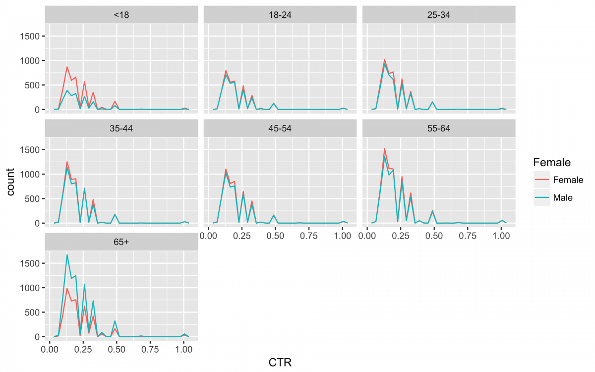
ggsave("nyt_data_freqpoly_CTR.png", width = 8, height = 5, unit = "in", dpi = 480)
There you have it! 31 clean data sets and a visualization in under 250 lines!!!!
- Getting started with stringr for textual analysis in R - February 8, 2024
- How to calculate a rolling average in R - June 22, 2020
- Update: How to geocode a CSV of addresses in R - June 13, 2020


Thank you so much! This was exactly what I needed and much easier to follow than solutions on StackOverflow!